For the complete documentation index, see llms.txt. This page is also available as Markdown.

How to use Google Sheets in a metric

Add Google Sheets data to journey-map metric cards by picking a spreadsheet, sheet, and the columns to plot.

Turn a column of values in a Google Sheet into a live chart or number on any journey map.

Prerequisites

Add a Google Sheets metric

You can create a Google Sheets metric from two places:

  • From the workspace Metrics tab - Click Metrics in the sidebar, then + Create metric. The full-page Add metric form opens.

  • From a journey map - Click + Add card on a card slot and pick Metric under Advanced cards. In the Add metric picker, pick an existing metric or type a name and click Create. The metric opens in a compact modal; use Full screen view to switch to the full-page form.

The steps below walk the workspace-tab flow because the full-page form shows every field on screen. The journey map modal has the same fields in a more compact layout.

1

Name the metric and pick Google Sheet as the source

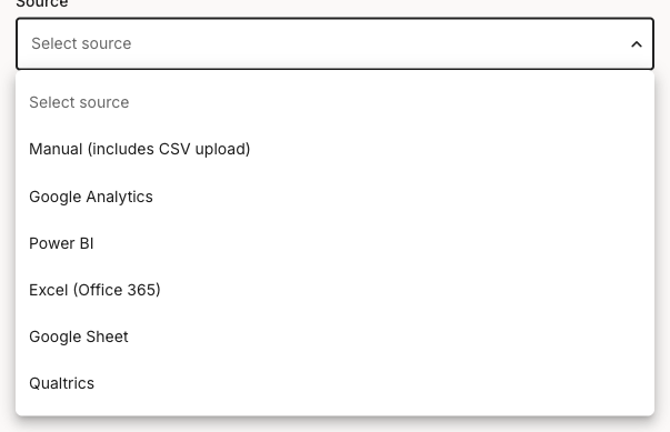
Type a name that describes what the metric shows (for example, New users by week). In Source, pick Google Sheet. The source list labels this option in the singular, Google Sheet, even though the integration itself is Google Sheets.

Source dropdown open on the Add metric form, listing Manual (includes CSV upload), Google Analytics, Power BI, Excel (Office 365), Google Sheet, and Qualtrics.
Source dropdown, Google Sheet selected

If you see a setup-required block below the Source field instead of the Sheets fields, the integration isn't connected for this account yet. Follow How to set up the Google Sheets integration before continuing.

2

Pick the metric type

Open the Type dropdown and pick Series, Number, or Comparison. The fields below depend on this choice. A Series plots a column of values as a chart, a Number shows a single headline value, and a Comparison sets two values against each other. The steps below walk a Series, the most common choice for sheet data.

3

Choose the spreadsheet and sheet

Click Select file under Spreadsheet and choose the Google Sheet to pull from. Then open the Sheet dropdown and pick which tab inside that file to read.

Add metric form with Source set to Google Sheet and Type set to Series. The left column shows Name, Source, Type, a Spreadsheet field with a Select file button, a Sheet dropdown, a Make top row headers checkbox under Header, Data label and Data values column dropdowns, a Select bottom rows checkbox under Row selection, and a Number of rows (max 50) field. The right column shows the Default card preview.
Add metric, Google Sheet fields
4

Map the columns to the chart

Turn on Make top row headers if the first row of the sheet holds column names, so Smaply reads row 1 as headers rather than data. The Data label and Data values dropdowns then list columns by name.

  • Pick the column for the chart's categories under Data label (for example, a Week column).

  • Pick the numeric column to plot under Data values (for example, a Users column).

For a field-by-field reference, see Field mapping below.

5

Set which rows to pull

Under Number of rows, set how many rows to read from the sheet. The maximum is 50.

Leave Select bottom rows off to read from the top of the sheet down. Turn it on to read the last rows instead, which is how you grab the most recent entries when new data is appended to the end of a long sheet.

6

Pick chart options and save

In the Default card preview panel on the right, pick a default chart type from the chip strip and add an optional Chart heading and Chart subheading. The preview updates as you change the selections. These are the defaults for new cards built from this metric; each card can override them on a journey map. For the full chart-options reference, see How to create and configure a metric.

Click Save. The metric appears in the workspace Metrics list and is ready to drop onto any journey map as a metric card.


Field mapping

Each field in the Add metric form points at part of your sheet. Work down the form in order, since the column dropdowns only list names once the spreadsheet, sheet, and header setting above them are set.

  • Spreadsheet - The Google Sheet file to pull from. Click Select file to choose it.

  • Sheet - The tab inside that file to read. A spreadsheet can hold several sheets, so pick the one with your data.

  • Make top row headers - Turn on when the first row holds column names. Smaply then treats row 1 as headers and lists your columns by name in the two fields below, rather than reading row 1 as data.

  • Data label - The column whose values become the categories on the chart (the x-axis on a bar or line chart, the slice labels on a pie chart). Example: a Week column with values like Week 1, Week 2, Week 3.

  • Data values - The numeric column whose values get plotted. Example: a Users column with the count per week.

  • Select bottom rows - Off reads rows from the top of the sheet; on reads them from the bottom. Use it with Number of rows to grab the most recent entries when new data is added to the end of the sheet.

  • Number of rows - Caps how many rows the metric pulls. Maximum 50.


Refresh behaviour

Google Sheets metrics refresh on access. When you open the workspace Metrics section or a journey map containing the metric, Smaply pulls fresh values if the last update was more than about an hour ago. Data under an hour old isn't re-pulled, and there's no manual refresh button. The next time you open the metric or its map brings the values up to date.

The metric reflects whatever the sheet held at the last pull, so an edit you just made in Google Sheets shows up on the next on-access refresh once the hour window has passed.

lightbulb

Tip: Shape the sheet to match the journey


Troubleshooting

If the connection itself isn't working, see How to set up the Google Sheets integration for connection troubleshooting. The issues below cover data-side problems once the connection is in place.

Metric shows no data or the columns are empty - Header or column mapping

The metric saves but the chart is blank, or the Data label and Data values dropdowns have nothing to pick.

  • Check that Make top row headers matches the sheet. If the first row holds column names but the toggle is off (or the reverse), Smaply reads the columns wrong and the value column won't map.

  • Confirm Data values points at a clean numeric column. Text, blanks, or mixed values in that column show as no data.

  • Confirm the chosen Sheet is the tab that actually holds the data, not an empty or summary tab in the same file.

Only part of the data shows, or the wrong rows show - Row cap or row direction

The chart renders but is missing rows you expected, or shows older entries instead of recent ones.

  • The Number of rows cap is 50. If the sheet has more rows than that, only the first (or last) 50 are pulled.

  • If the newest entries are at the bottom of the sheet and you want those, turn on Select bottom rows so the metric reads from the end rather than the top.

A metric that worked before stopped pulling - Spreadsheet or column changed

A metric that previously rendered starts returning errors or no data.

If the spreadsheet was renamed, moved, a sheet tab was renamed, or the Data label or Data values column was removed or reordered, the metric's references break until they're re-pointed. Edit the metric, re-pick the spreadsheet, sheet, and columns, and save. For service-account connections, also confirm the spreadsheet is still shared with the service-account email.

For wider questions about how integrations behave across tools (refresh frequency, switching auth, what happens on disconnect), see How to manage integrations.

Still not working? Contact support at help@smaply.com


Last updated